
Machine Learning (ML) Methoden sind eng verknüpft mit Optimierungsverfahren. Im ML wird in der Regel eine Zielfunktion definiert, deren Optimum mittels Optimierungsalgorithmus ermittelt werden muss. Auch zur Verbesserung von ML Methoden kann Optimierung verwendet werden, z.B. bei der Feature Selection (ein Anwendungsbeispiel gibt es unten im Beitrag). Daneben können Optimierungsmethoden auch im Operations Research eingesetzt werden, um komplexe, mathematisch formulierte Probleme z.B. aus dem Bereich Supply Chain- und Logistik-Optimierung zu lösen.
Die Statistikumgebung R besitzt viele in Paketen organisierte Erweiterungen, unter anderem eine Implementierung des genetischen Algorithmus im R Paket GA. Der genetische Algorithmus (GA) gehört zu den stochastischen Verfahren der Optimierungsmethoden. Dabei versucht der GA im Gegensatz zu den deterministischen Verfahren, nicht ein exaktes Optimum zu ermitteln. Deterministische Alorithmen haben dabei nämlich oft das Problem, dass anstelle eines globalen Optimums (siehe Grafik Punkt A) teilweise nur ein lokales Optimum (siehe Grafik Punkt B) ermittelt wird. Dabei sind die Rechenzeiten zur Lösungsermittlung teilweise sehr lang, denn es wird versucht, den gesamten Lösungsraum (in der Grafik die x-Achse von -1 bis 14) zu durchsuchen. Stochastische Verfahren betrachten häufig nicht den gesamten möglichen Lösungsraum, um darin die optimale Lösung zu finden, sondern nur einen Teil. Das hat zur Folge, dass bei reduzierter Berechnungszeit eine Approximation an ein globales Optimum möglich ist.

Prinzip und Grundstruktur des GAs
Der genetische Algorithmus orientiert sich am Prinzip der Evolution (“Survival of the fittest”), die dafür sorgt, dass Individuen mit den größeren Überlebenschancen ihre Eigenschaften an Nachkommen weitergeben können. Die Information zu Eigenschaften der Individuen werden dabei im Erbgut in einer Menge von Chromosomen abgelegt.
Im GA wird das Individuum einem einzelnen Chromosom gleichgesetzt. Das Chromosom besteht aus Genen, wobei jedes einzelne Gen eine codierte Eigenschaft darstellt.
Schritte des GAs:
1. Kodierung eines zu optimierenden Problems
2. Erzeugung Anfangspopulation
3. Bewerte Fitneßgüte der erzeugten Individuen
Solange ein Abbruchkriterium nicht erfüllt ist, werden die folgenden Schritte wiederholt:
4. Durch Selektion werden Elternteile ausgewählt
5. Mittels genetischer Operatoren (Kreuzung von Chromosomen, Permutation von Genen) wird neue Population erzeugt
6. Bewertung der Fitneß der neuen Individuen
Der genetische Algorithmus besteht damit aus einer Kodierungsvorschrift für Lösungskandidaten, die vorgibt wie die Populationen zu erzeugen und darzustellen sind. Es wird eine Fitnessfunktion zur Bewertung der Individuen benötigt, die oft identisch zu der zu optimierenden Funktion ist, aber auch zusätzliche Nebenbedingungen o.ä. beinhalten kann. Unterschiedliche Auswahlverfahren existieren, wie Elternteile selektiert werden für die Erzeugung von Nachkommen. Parameter des Algorithmus, über die der Algorithmus variiert werden kann, sind unter anderem die Populationsgröße, aber auch die Mutationswahrscheinlichkeit eines Gens.
Der GA besitzt viele Anwendungsmöglichkeiten. Neben dem Einsatz z.B. in der Losgrößenplanung oder Produktionsplanung kann der GA auch zur Lösung des Problems des Handlungsreisenden oder zur Feature Selektion eingesetzt werden. Diese beiden Anwendungsbeispiele werden im folgenden mit dem R-Paket GA kurz gezeigt.
Anwendungsbeispiel 1: Travelling Salesman Problem (TSP)
n Städte sollen beliefert werden. Beispielsweise 21 europäische Städte (Athen, Barcelona, Brüssel, Calais, Cherbourg, Köln, Kopenhagen, Genf, Gibraltar, Hamburg, Hoek van Holland, Lissabon, Lyon, Madrid, Marseilles, Mailand, München, Paris, Rom, Stockholm, Wien).
Ziel ist es, alle Städte unter Berücksichtung einer minimalen Gesamtstrecke zu besuchen und am Ende wieder am Startpunkt anzukommen. Dafür wird zuerst eine Matrix benötigt mit den Distanzen zwischen den Städten. Ein kleiner Auszug aus der Matrix (die Daten eurodist stammen aus dem R Pakete datasets, Abstände in KM):
##           Athens Barcelona Brussels Calais Cherbourg Cologne
## Athens         0      3313     2963   3175      3339    2762
## Barcelona   3313         0     1318   1326      1294    1498
## Brussels    2963      1318        0    204       583     206
## Calais      3175      1326      204      0       460     409
## Cherbourg   3339      1294      583    460         0     785
## Cologne     2762      1498      206    409       785       0
Jedes Individuum der Population ist eine Tour, die aus einer Permutation der 21 Städte besteht, in welcher Reihenfolge diese besucht werden. Die Fitness-Funktion berücksichtigt nun die Länge der jeweiligen Tour. Da die Fitness-Funktion maximiert wird, ist der Kehrwert der Tourlänge die Fitnessfunktion, zur Minimierung der Gesamtkilometerzahl.
# Funktion zur Berechnung der Laenge einer gegebenen Tour
tour.distance <- function(tour, dist){
  tour  <- c(tour, tour[1])     # Startpunkt = Endpunkt
  route <- embed(tour, 2)[,2:1] # jede Zeile der aufgespannten Matrix:
                                # Start- zu Zielstadt
  sum(dist[route])              # Summe der Kilometer zwischen Start u. Ziel
}

# Fitness Funktion
fitness.tsp <- function(tour, ...){1/tour.distance(tour, ...)} # Kehrwert
Durchführung des GA, dazu wird zuerst das Paket GA geladen.
library(GA)
GA.tsp <- ga(type = "permutation", fitness = fitness.tsp, dist = D,
            lower = 1, upper =  attr(eurodist, "Size"), popSize = 50,
           maxiter = 5000, run = 500, pmutation = 0.2)
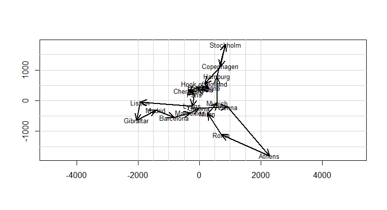
Ergebnis des GAs ist, dass die Städte in der folgenden Reihenfolge zu besuchen sind:
Munich, Cologne, Hamburg, Stockholm, Copenhagen, Hook of Holland, Calais, Brussels, Paris, Cherbourg, Madrid, Lisbon, Gibraltar, Barcelona, Marseilles, Lyons, Geneva, Milan, Rome, Athens, Vienna.
Anwendungsbeispiel 2: Feature Subset Selection
Eine Aufgabe im ML und der Statistik ist es, Variablen zu identifzieren, die am meisten relevant sind für die Erklärung eines Zusammenhangs. Damit folgt man dem Principle of Parsimony: Reduktion von nicht relevanter Komplexität. Interpretationen werden vereinfacht und Schätzungen verbessert.
Die Fitness eines Modells kann dabei mit unterschiedlichen Modellselektionskriteriern bewertet werden, z.B. bei Regressionsmodellen Akaike’s Information Criterium (AIC, Akaike 1973). Die Problemformulierung findet dann wie folgt statt, dass jeder Prädiktor des Modells mit einer binären Variablen dargestellt wird, je nachdem ob er Teil des Modells ist oder nicht.
Als Beispiel werden 100 normalverteilte Variablen simuliert, um damit ein lineares Regressionsmodell zur Erklärung des Zusammenhangs zur Variablen y zu schätzen. Aufgrund der Simulation ist bekannt, dass nur für einen Teil der Variablen ein Zusammenhang mit y besteht.
# set.seed(123)# 500 Beobachtungen von 100 normalverteilten Variablen M <- matrix(rnorm(500*100), ncol = 100) # zufällig erzeugte Regressionskoeffizienten b + Modellkonstante b1 b1 <- runif(1, min = 1, max = 10) b <- runif(100, min = 1, max = 10)my.mod <- lm(y ~ M[,id]) # es sollen nur ca. die Hälfte der Variablen in M die Variable y erklären # zufällige Auswahl der Variablen in d d <- rbinom(100,1,0.5) # simulierte abhängige Variable y mit normalverteiltem Fehlerterm y <- b1 + M[,which(d == 1)] %*% b[which(d == 1)] + runif(500, 0, .1)
In der Realität muss ein gutes Modell ohne Kenntnisse der wahren Zusammenhänge geschätzt werden – sonst müsste nicht geschätzt werden 🙂 Dabei können Algorithmen wie “Forward Stepwise Selection” oder “Backward Stepwise Selection” verwendet werden. Das bedeutet, dass entweder mit einem Modell ohne eine einzige erklärende Variable oder einem Modell mit allen zur Verfügung stehenden Variablen gestartet und dann schrittweise entweder eine Variable hinzugefügt bzw. entfernt wird, die das Modell im Vergleich zu dem Modell einen Schritt vorher am meisten verbessert. Diese Verfahren haben den Nachteil, dass nicht alle möglichen Variablenkonstellationen für das Modell berücksichtigt werden. Daher soll der GA die Modellselektion durchführen und den gesamten Lösungsraum durchsuchen.
Für den GA wird eine Fitness Funktion benötigt, die ein lineares Modell mit denjenigen Variablen schätzt, die eine 1 an der Position im Vektor selection haben. Rückgabewert ist der negative AIC Wert des jeweiligen Modells.
# Fitness Funktion
fitness.select <- function(selection){
  id <- which( selection == 1)
  my.mod <- lm(y ~ M[,id])

  # AIC als Kriterium zur Modellselektion
  return (-AIC(my.mod))
  }
Der GA wird durchgeführt inkl. einer Zusammenfassung des Algorithmus mit dem Befehl summary().
GA.select <- ga("binary", fitness = fitness.select, nBits = ncol(M),
                     maxiter = 250, popSize = 100, pcrossover = 0.6 )
summary(GA.select)
## -- Genetic Algorithm -------------------
##
## GA settings:
## Type                  =  binary
## Population size       =  100
## Number of generations =  250
## Elitism               =  5
## Crossover probability =  0.6
## Mutation probability  =  0.1
##
## GA results:
## Iterations             = 250
## Fitness function value = 2091.304
## Solution =
##      x1 x2 x3 x4 x5 x6 x7 x8 x9 x10  ...  x99 x100
## [1,]  1  1  1  0  1  0  0  1  0   0         1    1
Das Hauptinteresse liegt darin, wie gut der GA die Modellselektion betrieben hat. Dazu wird der binäre Indikator aus der Simulation mit dem Indikator aus der Lösung verglichen. 84 Variablen werden richtig zugeordnet.
table(summary(GA.select)$solution == d)
##
## FALSE  TRUE
##    16    84
Da folgende Modell enthält die vom GA gewählten Modellvariablen.
my.mod <- lm(y ~ M[,which(summary(GA.select)$solution == 1)])
summary(my.mod)
##
## Call:
## lm(formula = y ~ M[, which(summary(GA.select)$solution == 1)])
##
## Residuals:
##       Min        1Q    Median        3Q       Max
## -0.066474 -0.021293  0.000549  0.020007  0.060918
##
## Coefficients:
##                                                 Estimate Std. Error
## (Intercept)                                     6.470756   0.001350
## M[, which(summary(GA.select)$solution == 1)]1   1.206982   0.001388
## M[, which(summary(GA.select)$solution == 1)]2   8.386834   0.001309
## M[, which(summary(GA.select)$solution == 1)]3   1.325147   0.001350
## M[, which(summary(GA.select)$solution == 1)]4   8.835134   0.001435
## M[, which(summary(GA.select)$solution == 1)]5   4.993426   0.001342
## M[, which(summary(GA.select)$solution == 1)]6   0.001725   0.001402
## M[, which(summary(GA.select)$solution == 1)]7   0.001949   0.001292
## M[, which(summary(GA.select)$solution == 1)]8   7.769725   0.001372
## M[, which(summary(GA.select)$solution == 1)]9  -0.002180   0.001283
## M[, which(summary(GA.select)$solution == 1)]10  0.001916   0.001347
## M[, which(summary(GA.select)$solution == 1)]11  1.334782   0.001366
## M[, which(summary(GA.select)$solution == 1)]12  4.200184   0.001322
## M[, which(summary(GA.select)$solution == 1)]13  9.239261   0.001327
## M[, which(summary(GA.select)$solution == 1)]14  0.003308   0.001341
## M[, which(summary(GA.select)$solution == 1)]15  0.001932   0.001342
## M[, which(summary(GA.select)$solution == 1)]16  2.323913   0.001343
## M[, which(summary(GA.select)$solution == 1)]17  4.145069   0.001316
## M[, which(summary(GA.select)$solution == 1)]18  7.637314   0.001366
## M[, which(summary(GA.select)$solution == 1)]19  1.765503   0.001380
## M[, which(summary(GA.select)$solution == 1)]20  6.877427   0.001393
## M[, which(summary(GA.select)$solution == 1)]21  0.003250   0.001398
## M[, which(summary(GA.select)$solution == 1)]22  1.408433   0.001326
## M[, which(summary(GA.select)$solution == 1)]23  1.645951   0.001355
## M[, which(summary(GA.select)$solution == 1)]24  3.681626   0.001287
## M[, which(summary(GA.select)$solution == 1)]25  9.951557   0.001363
## M[, which(summary(GA.select)$solution == 1)]26  9.393009   0.001290
## M[, which(summary(GA.select)$solution == 1)]27  9.624555   0.001324
## M[, which(summary(GA.select)$solution == 1)]28  4.695577   0.001344
## M[, which(summary(GA.select)$solution == 1)]29  9.125584   0.001295
## M[, which(summary(GA.select)$solution == 1)]30  6.558717   0.001259
## M[, which(summary(GA.select)$solution == 1)]31  4.883307   0.001316
## M[, which(summary(GA.select)$solution == 1)]32  4.938663   0.001371
## M[, which(summary(GA.select)$solution == 1)]33  8.843227   0.001365
## M[, which(summary(GA.select)$solution == 1)]34  0.001907   0.001303
## M[, which(summary(GA.select)$solution == 1)]35  5.582821   0.001351
## M[, which(summary(GA.select)$solution == 1)]36  3.524090   0.001358
## M[, which(summary(GA.select)$solution == 1)]37 -0.001897   0.001389
## M[, which(summary(GA.select)$solution == 1)]38  7.997175   0.001309
## M[, which(summary(GA.select)$solution == 1)]39  3.520559   0.001426
## M[, which(summary(GA.select)$solution == 1)]40  5.329374   0.001424
## M[, which(summary(GA.select)$solution == 1)]41  5.637443   0.001301
## M[, which(summary(GA.select)$solution == 1)]42  8.725614   0.001314
## M[, which(summary(GA.select)$solution == 1)]43 -0.001666   0.001346
## M[, which(summary(GA.select)$solution == 1)]44  9.656752   0.001434
## M[, which(summary(GA.select)$solution == 1)]45  0.001936   0.001398
## M[, which(summary(GA.select)$solution == 1)]46  7.742001   0.001313
## M[, which(summary(GA.select)$solution == 1)]47 -0.002907   0.001396
## M[, which(summary(GA.select)$solution == 1)]48  2.433171   0.001352
## M[, which(summary(GA.select)$solution == 1)]49  7.862858   0.001362
## M[, which(summary(GA.select)$solution == 1)]50  0.001242   0.001344
## M[, which(summary(GA.select)$solution == 1)]51  4.394821   0.001310
## M[, which(summary(GA.select)$solution == 1)]52  5.912215   0.001338
## M[, which(summary(GA.select)$solution == 1)]53  5.632878   0.001360
## M[, which(summary(GA.select)$solution == 1)]54  3.075113   0.001373
## M[, which(summary(GA.select)$solution == 1)]55  7.143441   0.001238
## M[, which(summary(GA.select)$solution == 1)]56  1.698640   0.001313
## M[, which(summary(GA.select)$solution == 1)]57  0.003610   0.001336
## M[, which(summary(GA.select)$solution == 1)]58 -0.002374   0.001346
## M[, which(summary(GA.select)$solution == 1)]59  1.803126   0.001361
## M[, which(summary(GA.select)$solution == 1)]60  6.411209   0.001435
## M[, which(summary(GA.select)$solution == 1)]61  1.674603   0.001394
## M[, which(summary(GA.select)$solution == 1)]62  8.086532   0.001316
## M[, which(summary(GA.select)$solution == 1)]63  0.003395   0.001258
##                                                 t value Pr(>|t|)
## (Intercept)                                    4793.544  < 2e-16 ***
## M[, which(summary(GA.select)$solution == 1)]1   869.760  < 2e-16 ***
## M[, which(summary(GA.select)$solution == 1)]2  6409.250  < 2e-16 ***
## M[, which(summary(GA.select)$solution == 1)]3   981.339  < 2e-16 ***
## M[, which(summary(GA.select)$solution == 1)]4  6156.672  < 2e-16 ***
## M[, which(summary(GA.select)$solution == 1)]5  3721.918  < 2e-16 ***
## M[, which(summary(GA.select)$solution == 1)]6     1.230  0.21924
## M[, which(summary(GA.select)$solution == 1)]7     1.508  0.13220
## M[, which(summary(GA.select)$solution == 1)]8  5661.206  < 2e-16 ***
## M[, which(summary(GA.select)$solution == 1)]9    -1.699  0.09008 .
## M[, which(summary(GA.select)$solution == 1)]10    1.423  0.15548
## M[, which(summary(GA.select)$solution == 1)]11  977.314  < 2e-16 ***
## M[, which(summary(GA.select)$solution == 1)]12 3176.109  < 2e-16 ***
## M[, which(summary(GA.select)$solution == 1)]13 6961.450  < 2e-16 ***
## M[, which(summary(GA.select)$solution == 1)]14    2.467  0.01402 *
## M[, which(summary(GA.select)$solution == 1)]15    1.439  0.15086
## M[, which(summary(GA.select)$solution == 1)]16 1730.902  < 2e-16 ***
## M[, which(summary(GA.select)$solution == 1)]17 3149.183  < 2e-16 ***
## M[, which(summary(GA.select)$solution == 1)]18 5588.987  < 2e-16 ***
## M[, which(summary(GA.select)$solution == 1)]19 1279.081  < 2e-16 ***
## M[, which(summary(GA.select)$solution == 1)]20 4936.776  < 2e-16 ***
## M[, which(summary(GA.select)$solution == 1)]21    2.324  0.02058 *
## M[, which(summary(GA.select)$solution == 1)]22 1062.469  < 2e-16 ***
## M[, which(summary(GA.select)$solution == 1)]23 1214.816  < 2e-16 ***
## M[, which(summary(GA.select)$solution == 1)]24 2859.641  < 2e-16 ***
## M[, which(summary(GA.select)$solution == 1)]25 7302.126  < 2e-16 ***
## M[, which(summary(GA.select)$solution == 1)]26 7279.314  < 2e-16 ***
## M[, which(summary(GA.select)$solution == 1)]27 7266.883  < 2e-16 ***
## M[, which(summary(GA.select)$solution == 1)]28 3493.977  < 2e-16 ***
## M[, which(summary(GA.select)$solution == 1)]29 7047.144  < 2e-16 ***
## M[, which(summary(GA.select)$solution == 1)]30 5207.876  < 2e-16 ***
## M[, which(summary(GA.select)$solution == 1)]31 3711.788  < 2e-16 ***
## M[, which(summary(GA.select)$solution == 1)]32 3602.642  < 2e-16 ***
## M[, which(summary(GA.select)$solution == 1)]33 6476.600  < 2e-16 ***
## M[, which(summary(GA.select)$solution == 1)]34    1.464  0.14395
## M[, which(summary(GA.select)$solution == 1)]35 4132.336  < 2e-16 ***
## M[, which(summary(GA.select)$solution == 1)]36 2595.082  < 2e-16 ***
## M[, which(summary(GA.select)$solution == 1)]37   -1.365  0.17287
## M[, which(summary(GA.select)$solution == 1)]38 6107.588  < 2e-16 ***
## M[, which(summary(GA.select)$solution == 1)]39 2468.196  < 2e-16 ***
## M[, which(summary(GA.select)$solution == 1)]40 3742.145  < 2e-16 ***
## M[, which(summary(GA.select)$solution == 1)]41 4333.982  < 2e-16 ***
## M[, which(summary(GA.select)$solution == 1)]42 6639.353  < 2e-16 ***
## M[, which(summary(GA.select)$solution == 1)]43   -1.237  0.21671
## M[, which(summary(GA.select)$solution == 1)]44 6735.240  < 2e-16 ***
## M[, which(summary(GA.select)$solution == 1)]45    1.385  0.16675
## M[, which(summary(GA.select)$solution == 1)]46 5896.498  < 2e-16 ***
## M[, which(summary(GA.select)$solution == 1)]47   -2.083  0.03785 *
## M[, which(summary(GA.select)$solution == 1)]48 1799.570  < 2e-16 ***
## M[, which(summary(GA.select)$solution == 1)]49 5774.999  < 2e-16 ***
## M[, which(summary(GA.select)$solution == 1)]50    0.924  0.35607
## M[, which(summary(GA.select)$solution == 1)]51 3353.853  < 2e-16 ***
## M[, which(summary(GA.select)$solution == 1)]52 4418.565  < 2e-16 ***
## M[, which(summary(GA.select)$solution == 1)]53 4140.404  < 2e-16 ***
## M[, which(summary(GA.select)$solution == 1)]54 2240.383  < 2e-16 ***
## M[, which(summary(GA.select)$solution == 1)]55 5772.231  < 2e-16 ***
## M[, which(summary(GA.select)$solution == 1)]56 1293.364  < 2e-16 ***
## M[, which(summary(GA.select)$solution == 1)]57    2.703  0.00715 **
## M[, which(summary(GA.select)$solution == 1)]58   -1.764  0.07851 .
## M[, which(summary(GA.select)$solution == 1)]59 1324.965  < 2e-16 ***
## M[, which(summary(GA.select)$solution == 1)]60 4467.123  < 2e-16 ***
## M[, which(summary(GA.select)$solution == 1)]61 1201.312  < 2e-16 ***
## M[, which(summary(GA.select)$solution == 1)]62 6145.354  < 2e-16 ***
## M[, which(summary(GA.select)$solution == 1)]63    2.699  0.00722 **
## ---
## Signif. codes:  0 '***' 0.001 '**' 0.01 '*' 0.05 '.' 0.1 ' ' 1
##
## Residual standard error: 0.02811 on 436 degrees of freedom
## Multiple R-squared:      1,  Adjusted R-squared:      1
## F-statistic: 1.609e+07 on 63 and 436 DF,  p-value: < 2.2e-16
Quellen
Akaike, H. (1973). Information Theory and an Extension of the Maximum Likelihood Principle. In B. N. Petrov, & F. Csaki (Eds.), Proceedings of the 2nd International Symposium on Information Theory (pp. 267-281). Budapest: Akademiai Kiado.
Scrucca, L. (2013). GA: A Package for Genetic Algorithms in R. Journal of
Statistical Software, 53(4), 1-37. URL http://www.jstatsoft.org/v53/i04/
